Solving Boundary Value Problems

In addition to finding solutions for an IVP and estimate the unknown parameters, this package also allows you to solve BVP with a little bit of imagination. Here, we are going to show how a BVP can be solved by treating it as a parameter estimation problem. Essentially, a shooting method where the first boundary condition defines the initial condition of an IVP and the second boundary condition is an observation. Two examples, both from MATLAB [1], will be shown here.

Simple model 1

We are trying to find the solution to the second order differential equation

\[\nabla^{2} y + |y| = 0\]

subject to the boundary conditions \(y(0) = 0\) and \(y(4) = -2\). Convert this into a set of first order ODE

\[\begin{split}\frac{d y_{0}}{dt} &= y_{1} \\ \frac{d y_{1}}{dt} &= -|y_{0}|\end{split}\]

using an auxiliary variable \(y_{1} = \nabla y\) and \(y_{0} = y\). Setting up the system below

In [1]: from pygom import Transition, TransitionType, DeterministicOde, SquareLoss

In [2]: import matplotlib.pyplot as plt

In [3]: stateList = ['y0', 'y1']

In [4]: paramList = []

In [5]: ode1 = Transition(origin='y0',
   ...:                   equation='y1',
   ...:                   transition_type=TransitionType.ODE)
   ...: 

In [6]: ode2 = Transition(origin='y1',
   ...:                   equation='-abs(y0)',
   ...:                   transition_type=TransitionType.ODE)
   ...: 

In [7]: model = DeterministicOde(stateList,
   ...:                          paramList,
   ...:                          ode=[ode1, ode2])
   ...: 

In [8]: model.get_ode_eqn()
Out[8]: 
Matrix([
[      y1],
[-Abs(y0)]])

We check that the equations are correct before proceeding to set up our loss function.

In [9]: import numpy

In [10]: from scipy.optimize import minimize

In [11]: initialState = [0.0, 1.0]

In [12]: t = numpy.linspace(0, 4, 100)

In [13]: model.initial_values = (initialState, t[0])

In [14]: solution = model.integrate(t[1::])

In [15]: f = plt.figure()

In [16]: model.plot()

In [17]: plt.close()

Setting up the second boundary condition \(y(4) = -2\) is easy, because that is just a single observation attached to the state \(y_{1}\). Enforcing the first boundary condition requires us to set it as the initial condition. Because the condition only states that \(y(0) = 0\), the starting value of the other state \(y_1\) is free. We let our loss object know that it is free through the targetState input argument.

In [18]: theta = [0.0]

In [19]: obj = SquareLoss(theta=theta,
   ....:                  ode=model,
   ....:                  x0=initialState,
   ....:                  t0=t[0],
   ....:                  t=t[-1],
   ....:                  y=[-2],
   ....:                  state_name=['y0'],
   ....:                  target_state=['y1'])
   ....: 

In [20]: thetaHat = minimize(fun=obj.costIV, x0=[0.0])

In [21]: print(thetaHat)
      fun: 1.8896300643324946e-11
 hess_inv: array([[0.51403884]])
      jac: array([-8.6096985e-06])
  message: 'Optimization terminated successfully.'
     nfev: 18
      nit: 5
     njev: 6
   status: 0
  success: True
        x: array([2.06657723])

In [22]: model.initial_values = ([0.0] + thetaHat['x'].tolist(), t[0])

In [23]: solution = model.integrate(t[1::])

In [24]: f = plt.figure()

In [25]: model.plot()

In [26]: plt.close()

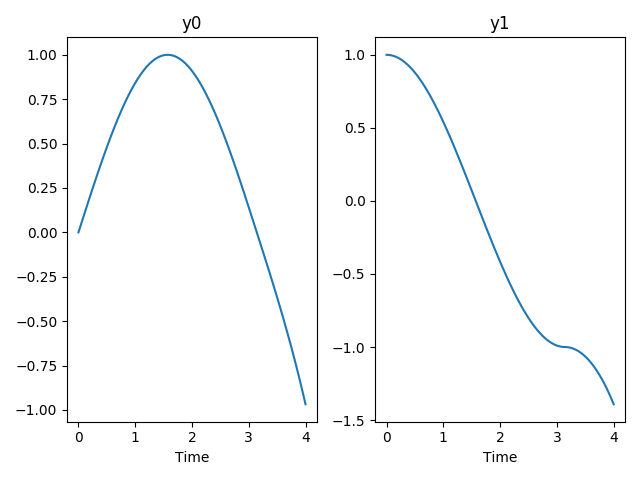
We are going to visualize the solution, and also check the boundary condition. The first became our initial condition, so it is always satisfied and only the latter is of concern, which is zero (subject to numerical error) from thetaHat.

Simple model 2

Our second example is different as it involves an actual parameter and also time. We have the Mathieu’s Equation

\[\nabla^{2} y + \left(p - 2q \cos(2x)\right)y = 0\]

and the aim is to compute the fourth eigenvalue \(q=5\). There are three boundary conditions

\[\nabla y(0) = 0, \quad \nabla y(\pi) = 0, \quad y(0) = 1\]

and we aim to solve it by converting it to a first order ODE and tackle it as an IVP. As our model object does not allow the use of the time component in the equations, we introduce a anxiliary state \(\tau\) that replaces time \(t\). Rewrite the equations using \(y_{0} = y, y_{1} = \nabla y\) and define our model as

In [27]: stateList = ['y0', 'y1', 'tau']

In [28]: paramList = ['p']

In [29]: ode1 = Transition('y0', 'y1', TransitionType.ODE)

In [30]: ode2 = Transition('y1', '-(p - 2*5*cos(2*tau))*y0', TransitionType.ODE)

In [31]: ode3 = Transition('tau', '1', TransitionType.ODE)

In [32]: model = DeterministicOde(stateList, paramList, ode=[ode1, ode2, ode3])

In [33]: theta = [1.0, 1.0, 0.0]

In [34]: p = 15.0

In [35]: t = numpy.linspace(0, numpy.pi)

In [36]: model.parameters = [('p',p)]

In [37]: model.initial_values = (theta, t[0])

In [38]: solution = model.integrate(t[1::])

In [39]: f = plt.figure()

In [40]: model.plot()

In [41]: plt.close()

Now we are ready to setup the estimation. Like before, we setup the second boundary condition by pretending that it is an observation. We have all the initial conditions defined by the first boundary condition

In [42]: obj = SquareLoss(15.0, model, x0=[1.0, 0.0, 0.0], t0=0.0, t=numpy.pi, y=0.0, state_name='y1')

In [43]: xhatObj = minimize(obj.cost,[15])

In [44]: print(xhatObj)
      fun: 8.620622377669915e-17
 hess_inv: array([[0.41085766]])
      jac: array([-2.35234683e-09])
  message: 'Optimization terminated successfully.'
     nfev: 27
      nit: 5
     njev: 9
   status: 0
  success: True
        x: array([17.09658168])

In [45]: model.parameters = [('p', xhatObj['x'][0])]

In [46]: model.initial_values = ([1.0, 0.0, 0.0], t[0])

In [47]: solution = model.integrate(t[1::])

In [48]: f = plt.figure()

In [49]: model.plot()

In [50]: plt.close()

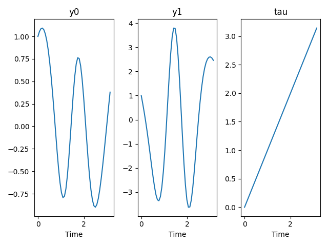
The plot of the solution shows the path that satisfies all boundary condition. The last subplot is time which obvious is redundant here but the DeterministicOde.plot() method is not yet able to recognize the time component. Possible speed up can be achieved through the use of derivative information or via root finding method that tackles the gradient directly, instead of the cost function.

Reference

[1]	http://uk.mathworks.com/help/matlab/ref/bvp4c.html