Stochastic representation of ode
There are multiple interpretation of stochasticity of a deterministic ode. We have implemented two of the most common interpretation; when the parameters are realizations of some underlying distribution, and when we have a so called chemical master equation where each transition represent a jump. Again, we use the standard SIR example as previously seen in ref:sir.
In [1]: from pygom import SimulateOde, Transition, TransitionType

In [2]: import matplotlib.pyplot as plt

In [3]: import numpy as np

In [4]: x0 = [1, 1.27e-6, 0]

In [5]: t = np.linspace(0, 150, 100)

In [6]: stateList = ['S', 'I', 'R']

In [7]: paramList = ['beta', 'gamma']

In [8]: transitionList = [
   ...:                   Transition(origin='S', destination='I', equation='beta*S*I', transition_type=TransitionType.T),
   ...:                   Transition(origin='I', destination='R', equation='gamma*I', transition_type=TransitionType.T)
   ...:                   ]
   ...:

In [9]: odeS = SimulateOde(stateList, paramList, transition=transitionList)

In [10]: odeS.parameters = [0.5, 1.0/3.0]

In [11]: odeS.initial_values = (x0, t[0])

In [12]: solutionReference = odeS.integrate(t[1::], full_output=False)
Stochastic Parameter
In our first scenario, we assume that the parameters follow some underlying distribution. Given that both \(\beta\) and \(\gamma\) in our SIR model has to be non-negative, it seemed natural to use a Gamma distribution. We make use of the familiar syntax from R to define our distribution. Unfortunately, we have to define it via a tuple, where the first is the function handle (name) while the second the parameters. Note that the parameters can be defined as either a dictionary or as the same sequence as R, which is the shape then the rate in the Gamma case.
In [13]: from pygom.utilR import rgamma

In [14]: d = dict()

In [15]: d['beta'] = (rgamma,{'shape':100.0, 'rate':200.0})

In [16]: d['gamma'] = (rgamma,(100.0, 300.0))

In [17]: odeS.parameters = d

In [18]: Ymean, Yall = odeS.simulate_param(t[1::], 10, full_output=True)
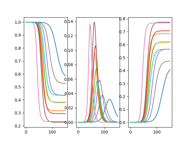
Note that a message is printed above where it is trying to connect to an mpi backend, as our module has the capability to compute in parallel using the IPython. We have simulated a total of 10 different solutions using different parameters, the plots can be seen below
In [19]: f, axarr = plt.subplots(1,3)

In [20]: for solution in Yall:
   ....:     axarr[0].plot(t, solution[:,0])
   ....:     axarr[1].plot(t, solution[:,1])
   ....:     axarr[2].plot(t, solution[:,2])
   ....:

In [21]: plt.show()

In [22]: plt.close()
We then see how the expected results, using the sample average of the simulations
differs from the reference solution
In [23]: f, axarr = plt.subplots(1,3)

In [24]: for i in range(3): axarr[i].plot(t, Ymean[:,i] - solutionReference[:,i])

In [25]: plt.show()

In [26]: plt.close()

The difference is relatively large especially for the \(S\) state. We can decrease this difference as we increase the number of simulation, and more sophisticated sampling method for the generation of random variables can also decrease the difference.
In addition to using the built-in functions to represent stochasticity, we can also use standard frozen distributions from scipy. Note that it must be a frozen distribution as that is the only for the parameters of the distributions to propagate through the model.
In [27]: import scipy.stats as st

In [28]: d = dict()

In [29]: d['beta'] = st.gamma(a=100.0, scale=1.0/200.0)

In [30]: d['gamma'] = st.gamma(a=100.0, scale=1.0/300.0)

In [31]: odeS.parameters = d
Obviously, there may be scenarios where only some of the parameters are stochastic. Let’s say that the \(\gamma\) parameter is fixed at \(1/3\), then simply replace the distribution information with a scalar. A quick visual inspection at the resulting plot suggests that the system of ODE potentially has less variation when compared to the case where both parameters are stochastic.
In [32]: d['gamma'] = 1.0/3.0

In [33]: odeS.parameters = d

In [34]: YmeanSingle, YallSingle = odeS.simulate_param(t[1::], 5, full_output=True)

In [35]: f, axarr = plt.subplots(1,3)

In [36]: for solution in YallSingle:
   ....:     axarr[0].plot(t,solution[:,0])
   ....:     axarr[1].plot(t,solution[:,1])
   ....:     axarr[2].plot(t,solution[:,2])
   ....:

In [37]: plt.show()

In [38]: plt.close()

Continuous Markov Representation
Another common method of introducing stochasticity into a set of ode is by assuming each movement in the system is a result of a jump process. More concretely, the probabilty of a move for transition \(j\) is governed by an exponential distribution such that
where \(\lambda_{j}\) is the rate of transition for process \(j\) and \(\tau\) the time elapsed after current time \(t\).
A couple of the commmon implementation for the jump process have been implemented where two of them are used during a normal simulation; the first reaction method [Gillespie1977] and the \(\tau\)-Leap method [Cao2006]. The two changes interactively depending on the size of the states.
In [39]: x0 = [2362206.0, 3.0, 0.0]

In [40]: stateList = ['S', 'I', 'R']

In [41]: paramList = ['beta', 'gamma', 'N']

In [42]: transitionList = [
   ....:                   Transition(origin='S', destination='I', equation='beta*S*I/N', transition_type=TransitionType.T),
   ....:                   Transition(origin='I', destination='R', equation='gamma*I', transition_type=TransitionType.T)
   ....:                   ]
   ....:

In [43]: odeS = SimulateOde(stateList, paramList, transition=transitionList)

In [44]: odeS.parameters = [0.5, 1.0/3.0, x0[0]]

In [45]: odeS.initial_values = (x0, t[0])

In [46]: solutionReference = odeS.integrate(t[1::])

In [47]: simX, simT = odeS.simulate_jump(t[1:10], 10, full_output=True)

In [48]: f, axarr = plt.subplots(1, 3)

In [49]: for solution in simX:
   ....:     axarr[0].plot(t[:9], solution[:,0])
   ....:     axarr[1].plot(t[:9], solution[:,1])
   ....:     axarr[2].plot(t[:9], solution[:,2])
   ....:

In [50]: plt.show()

In [51]: plt.close()

Above, we see ten different simulation, again using the SIR model but without standardization of the initial conditions. We restrict our time frame to be only the first 10 time points so that the individual changes can be seen more clearly above. If we use the same time frame as the one used previously for the deterministic system (as shown below), the trajectories are smoothed out and we no longer observe the jumps. Looking at the raw trajectories of the ODE below, it is obvious that the mean from a jump process is very different to the deterministic solution. The reason behind this is that the jump process above was able to fully remove all the initial infected individuals before any new ones.
In [52]: simX,simT = odeS.simulate_jump(t, 5, full_output=True)

In [53]: simMean = np.mean(simX, axis=0)

In [54]: f, axarr = plt.subplots(1,3)

In [55]: for solution in simX:
   ....:     axarr[0].plot(t, solution[:,0])
   ....:     axarr[1].plot(t, solution[:,1])
   ....:     axarr[2].plot(t, solution[:,2])
   ....:

In [56]: plt.show()

In [57]: plt.close()

Repeatable Simulation
One of the possible use of compartmental models is to generate forecasts. Although most of the time the requirement would be to have (at least point-wise) convergence in the limit, reproducibility is also important. For both types of interpretation explained above, we have given the package the capability to repeat the simulations by setting a seed. When the assumption is that the parameters follows some sort of distribution, we simply set the seed which governs the global state of the random number generator.
In [58]: x0 = [2362206.0, 3.0, 0.0]

In [59]: odeS = SimulateOde(stateList, paramList, transition=transitionList)

In [60]: d = {'beta': st.gamma(a=100.0, scale=1.0/200.0), 'gamma': st.gamma(a=100.0, scale=1.0/300.0), 'N': x0[0]}

In [61]: odeS.parameters = d

In [62]: odeS.initial_values = (x0, t[0])

In [63]: Ymean, Yall = odeS.simulate_param(t[1::], 10, full_output=True)

In [64]: np.random.seed(1)

In [65]: Ymean1, Yall1 = odeS.simulate_param(t[1::], 10, full_output=True)

In [66]: np.random.seed(1)

In [67]: Ymean2, Yall2 = odeS.simulate_param(t[1::], 10, full_output=True)

In [68]: sim_diff = [np.linalg.norm(Yall[i] - yi) for i, yi in enumerate(Yall1)]

In [69]: sim_diff12 = [np.linalg.norm(Yall2[i] - yi) for i, yi in enumerate(Yall1)]

In [70]: print("Different in the simulations and the mean: (%s, %s) " % (np.sum(sim_diff), np.sum(np.abs(Ymean1 - Ymean))))
Different in the simulations and the mean: (105510847.861041, 80664436.28054059)

In [71]: print("Different in the simulations and the mean using same seed: (%s, %s) " % (np.sum(sim_diff12), np.sum(np.abs(Ymean2 - Ymean1))))
Different in the simulations and the mean using same seed: (0.0, 0.0)
In the alternative interpretation, setting the global seed is insufficient. Unlike simulation based on the parameters, where we can pre-generate all the parameter values and send them off to individual processes in the parallel backend, this is prohibitive here. In a nutshell, the seed does not propagate when using a parallel backend because each integration requires an unknown number of random samples. Therefore, we have an additional flag parallel in the function signature. By ensuring that the computation runs in serial, we can make use of the global seed and generate identical runs.
In [72]: x0 = [2362206.0, 3.0, 0.0]

In [73]: odeS = SimulateOde(stateList, paramList, transition=transitionList)

In [74]: odeS.parameters = [0.5, 1.0/3.0, x0[0]]

In [75]: odeS.initial_values = (x0, t[0])

In [76]: simX, simT = odeS.simulate_jump(t[1:10], 10, parallel=False, full_output=True)

In [77]: np.random.seed(1)

In [78]: simX1, simT1 = odeS.simulate_jump(t[1:10], 10, parallel=False, full_output=True)

In [79]: np.random.seed(1)

In [80]: simX2, simT2 = odeS.simulate_jump(t[1:10], 10, parallel=False, full_output=True)

In [81]: sim_diff = [np.linalg.norm(simX[i] - x1) for i, x1 in enumerate(simX1)]

In [82]: sim_diff12 = [np.linalg.norm(simX2[i] - x1) for i, x1 in enumerate(simX1)]

In [83]: print("Difference in simulation: %s" % np.sum(np.abs(sim_diff)))
Difference in simulation: 2534.4614923250074

In [84]: print("Difference in simulation using same seed: %s" % np.sum(np.abs(sim_diff12)))
Difference in simulation using same seed: 0.0